Profile Parametric Node¶

Profile Node implements a useful subset of the SVG path section commands (see SVG specification). Used domain-specific language (DSL) is based on SVG specification, but does not exactly follow it, by adding some extensions and not supporting some features.

Profile definition consists of a series of statements (also called commands).

Statements may optionally be separated by semicolons (;). For some commands (namely: H/h, V/v, @i) the trailing semicolon is required!

There are the following statements supported:

“default” statement: default <name> = <value>. Here <name> is any valid python variable identifier, and <value> is a number or expression (see below). This statement declares a default value for the variable; this value will be used if corresponding input of the node is not connected.
“let” statement: let <name> = <value>. Here <name> is any valid python variable identifier, and <value> is a number or expression (see below). This statement declares a “name binding”; it may be used to calculate some value once and use it in the following statements several times. Variables defined by “let” statements will not appear as node inputs.
Line and curve segment commands - see the table below for details.

The following segment types are available:

name	cmd	parameters
MoveTo	M, m	<2v coordinate>
LineTo	L, l	(<2v coordinate>)+ [“n = “ num_segments] [z]
HorLineTo	H, h	(<x>)+ [“n = “ num_segments] “;”
VertLineTo	V, v	(<y>)+ [“n = “ num_segments] “;”
CurveTo	C, c	(<2v control1> <2v control2> <2v knot2>)+ [“n = “ num_verts] [z]
SmoothCurveTo	S, s	(<2v control2> <2v knot2>)+ [“n = “ num_verts] [z]
QuadCurveTo	Q, q	(<2v control> <2v knot2>)+ [“n = “ num_segments] [z]
SmthQuadCurve	T, t	(<2v knot2>)+ [“n = “ num_segments] [z]
ArcTo	A, a	<2v rx,ry> <float rot> <int flag1> <int flag2> <2v x,y> [“n = “ num_verts] [z]
Interpolate	@I, @i	[“@smooth”] <degree> (<2v point>)+ [“n = “ num_segments] [z] “;”
ClosePath	x
CloseAll	X
comment	#	anything after # is a comment.

<>  : mandatory field
[]  : optional field
2v  : two point vector `a,b`
        - no backticks
        - a and b can be
            - number literals
            - lowercase 1-character symbols for variables
(...)+ : this sequence may appear several times
int : means the value will be cast as an int even if you input float
      flags generally are 0 or 1.
["n = " num_verts] : for curve and line commands, number of subdivisions may be specified.
      For curve commands, default number of segments is specified in node settings (in the N panel).
      For line commands, default number of segments is always 1.
z   : is optional for closing a line
X   : as a final command to close the edges (cyclic) [-1, 0]
      in addition, if the first and last vertex share coordinate space
      the last vertex is dropped and the cycle is made anyway.
#   : single line comment prefix

Commands starting with capital letters (M, L, C, A) define all coordinates in absolute mode. Commands starting with lower case letters (m, l, c, a) define all coordinates in relative mode, i.e. each coordinate is defined with relation to “current pen position”.

Each integer or floating value may be represented as

Integer or floating literal (usual python syntax, such as 5 or 7.5)
Variable name, such as a or b or variable_name
Negation sign and a variable name, such as -a or -size.
Expression enclosed in curly brackets, such as {a+1} or {sin(phi)}

ArcTo only take enough parameters to complete one Arc, unlike real SVG command which take a whole sequence of chained ArcTo commands. The decision to keep it at one segment type per line is mainly to preserve readability.

Other curve segments (C/c, S/s, Q/q, T/t) allow to draw several segments with one command, as well as in SVG; but still, in many cases it is a good idea to use one segment per command, for readability reasons.

@I / @i command is an extension of SVG syntax. It defines a curve as interpolating NURBS curve through the provided list of points. Current point, at which the pen is located at the start of command, will be considered as first point to be interpolated. If z is specified in the end, the curve will be closed (cyclic); otherwise, this command will define an open curve. If special keyword, @smooth, is specified, then, while computing interpolation curve, this command will consider previous curve segment, defined by previous command (C/c, S/s, Q/q, T/t), if it is of the same degree, and draw the curve in such a way that in the starting point it will have the same tangent vector, as previous curve had in the end point; in other words, at the meeting point of segments, the curve will be smooth. Providing z and @smooth for the same @i command is not supported.

All curve segment types allow you to specify how many vertices are used to generate the segment. SVG doesn’t let you specify such things, but it makes sense to allow it for the creation of geometry.

Note: “default” and “let” definitions may use previously defined variables, or variables expected to be provided as inputs. Just note that these statements are evaluated in the same order as they follow in the input profile text.

For examples, see “Examples of usage” section below, or profile_examples directory in Sverchok distribution.

Expression syntax¶

Syntax being used in profile definitions is standard Python’s syntax for expressions. For exact syntax definition, please refer to https://docs.python.org/3/reference/expressions.html.

In short, you can use usual mathematical operations (+, -, *, /, ** for power), numbers, variables, parenthesis, and function call, such as sin(x).

One difference with Python’s syntax is that you can call only restricted number of Python’s functions. Allowed are:

Functions from math module:
- acos, acosh, asin, asinh, atan, atan2, atanh, ceil, copysign, cos, cosh, degrees, erf, erfc, exp, expm1, fabs, factorial, floor, fmod, frexp, fsum, gamma, hypot, isfinite, isinf, isnan, ldexp, lgamma, log, log10, log1p, log2, modf, pow, radians, sin, sinh, sqrt, tan, tanh, trunc;
Constants from math module: pi, e;
Additional functions: abs;
From mathutlis module: Vector, Matrix;
Python type conversions: tuple, list.

This restriction is for security reasons. However, Python’s ecosystem does not guarantee that no one can call some unsafe operations by using some sort of language-level hacks. So, please be warned that usage of this node with profile definition obtained from unknown or untrusted source can potentially harm your system or data.

Examples of valid expressions are:

1.0
x
{x+1}
{0.75*X + 0.25*Y}
{R * sin(phi)}

Inputs¶

Set of inputs for this node depends on expressions used in the profile definition. Each variable used in profile (except ones declared with “let” statements) becomes one input. If there are no variables used in profile, then this node will have no inputs.

Parameters¶

This node has the following parameters:

Axis. Available values are X, Y, Z. This parameter specifies the plane in which the curve will be produced. For example, default value of Z means that all points will belong to XOY plane.
File name. Name of Blender text buffer, containing profile description.
Precision. Number of decimal places used for points coordinates when generating a profile by from selection operator. Default value is 8. This parameter is only available in the N panel.
Curve points count. Default number of points for curve segment commands. Default value is 20. This parameter is available only in the N panel.
X command threshold. This parameter provides control over “remove doubles” functionality of the X command: if the distance between last and first points is less than this threshold, X command will remove the last point and connect pre-last point to the first instead.
NURBS output. This parameter is available in the N panel only. If checked, then the node will output all curve objects as NURBS curves. Otherwise, it will output specific types of curves (lines, circles, Bezier curves). In many cases, there is no difference; NURBS curves can be usable to apply specific API methods, or to output the result to formats that understand NURBS only. Unchecked by default.
Concatenate. This parameter is available in the N panel only. If checked, then the node will concatenate curve objects it generates. The curves can be automatically split into groups before concatenation, according to which of their endpoints coincide. For example, if you defined several separate contours (each made of several segments / commands), you will have several Curve objects. If NURBS output parameter is checked too, then the node will output single NURBS curve for each contour. If not checked, the node will output separate Curve object for each segment (command). Unchecked by default.
Concat tolerance. This parameter is available in the N panel only, and only if Concatenate parameter is checked. This defines distance between end point of one curve and starting point of another curve, which the node will use to decide whether it is required to concatenate them. The default value is 0.0001.

Outputs¶

This node has the following outputs:

Vertices. Resulting curve vertices.
Edges. Edges of the resulting curve.
Knots. Knot points of all curve segments (C/c, S/s, Q/q, T/t commands) used in the profile.
KnotNames. Names of all knot points. This output in junction with Knots may be used to display all knots in the 3D view by use of Viewer Index node - this is very useful for debugging of your profile.
Curve. Curve objects generated. This output contains a separate Curve object for each segment (each instruction).

Operators¶

As you know there are three types of curves in Blender - Polylines, Bezier curves and NURBS curves. This node has one operator button: from selection. This operator works only with Bezier curves. It takes an active Curve object, generates profile description from it and sets up the node to use this generated profile. You can adjust the profile by editing created Blender’s text bufrfer.

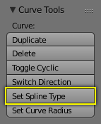
If you want to import other type of curve you have to convert one to Bezier type. Fortunately it is possible to do in edit mode with button Set Spline Type in the T panel. More information about conversion looks here.

One can also load one of examples, which are provided within Sverchok distribution. For that, in the N panel of Profile node, see “Profile templates” menu.

Examples¶

If you have experience with SVG paths most of this will be familiar. The biggest difference is that only the LineTo command accepts many points. It is a good idea to always start the profile with a M <pos>,<pos>.

M 0,0
L a,a b,0 c,0 d,d e,-e

the fun bit about this is that all these variables / components can be dynamic

M 0,0
L 0,3 2,3 2,4
C 2,5 2,5 3,5 n=10
L 5,5
C 7,5 7,5 7,3 n=10
L 7,2 5,0
X

or

M a,a
L a,b c,b -c,d
C c,e c,e b,e n=g
L e,e
C f,e f,e f,-b n=g
L f,c e,a
X

Examples of usage¶

The node started out as a thought experiment and turned into something quite useful, you can see how it evolved in the initial github thread ; See also last github thread and examples provided within Sverchok distribution (N panel of the node).

Example usage:

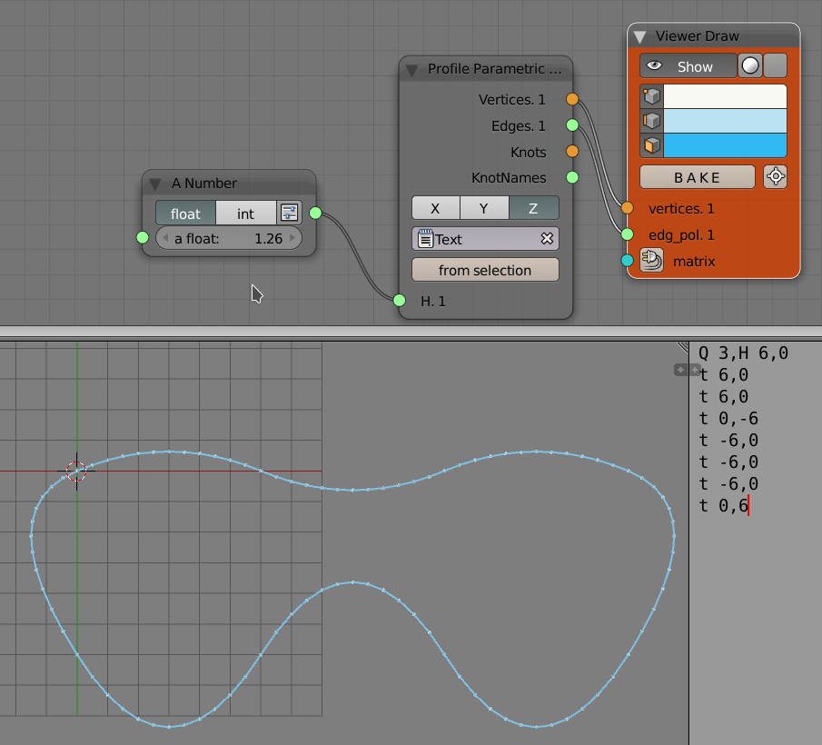
Q 3,H 6,0
t 6,0
t 6,0
t 0,-6
t -6,0
t -6,0
t -6,0
t 0,6

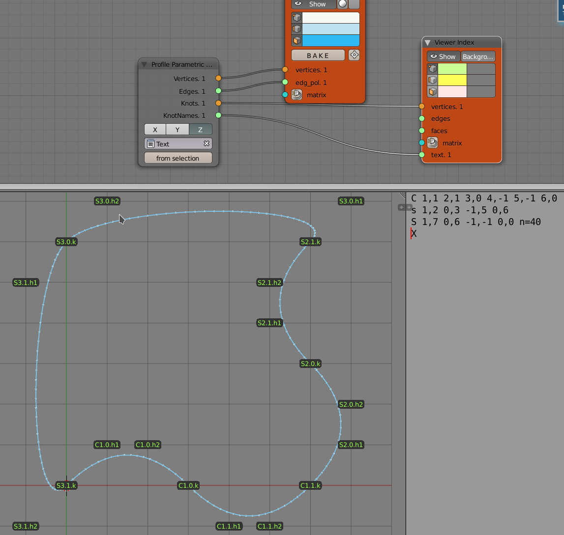
C 1,1 2,1 3,0 4,-1 5,-1 6,0
s 1,2 0,3 -1,5 0,6
S 1,7 0,6 -1,-1 0,0 n=40
X

An example with use of “default” and “let” statements:

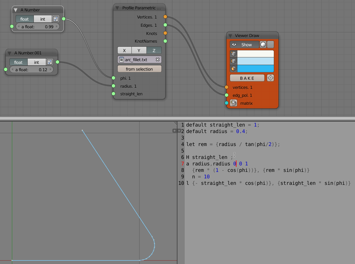
default straight_len = 1;
default radius = 0.4;

let rem = {radius / tan(phi/2)};

H straight_len ;
a radius,radius 0 0 1
  {rem * (1 - cos(phi))}, {rem * sin(phi)}
  n = 10
l {- straight_len * cos(phi)}, {straight_len * sin(phi)}

A simple example of @I command used to define a quadratic interpolation curve through three points:

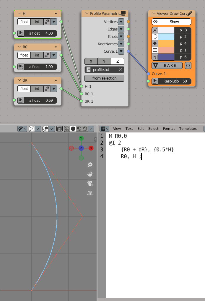
M R0,0
@I 2
   {R0 + dR}, {0.5*H}
   R0, H ;

An example of closed interpolation curve:

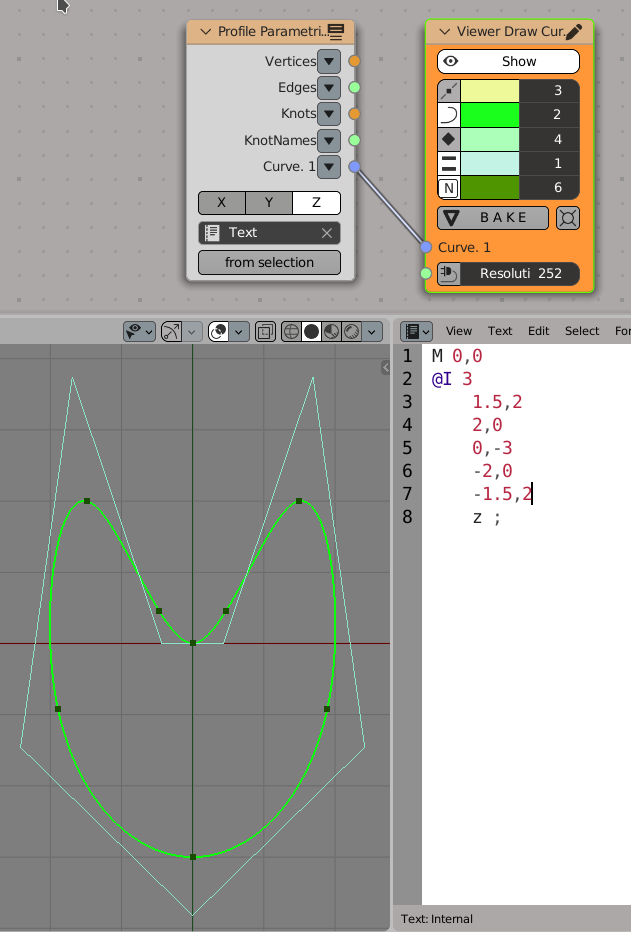
M 0,0
@I 3
   1.5,2
   2,0
   0,-3
   -2,0
   -1.5,2
   z ;

An example of @smooth keyword usage, to smoothly continue the previous segment defined by C command:

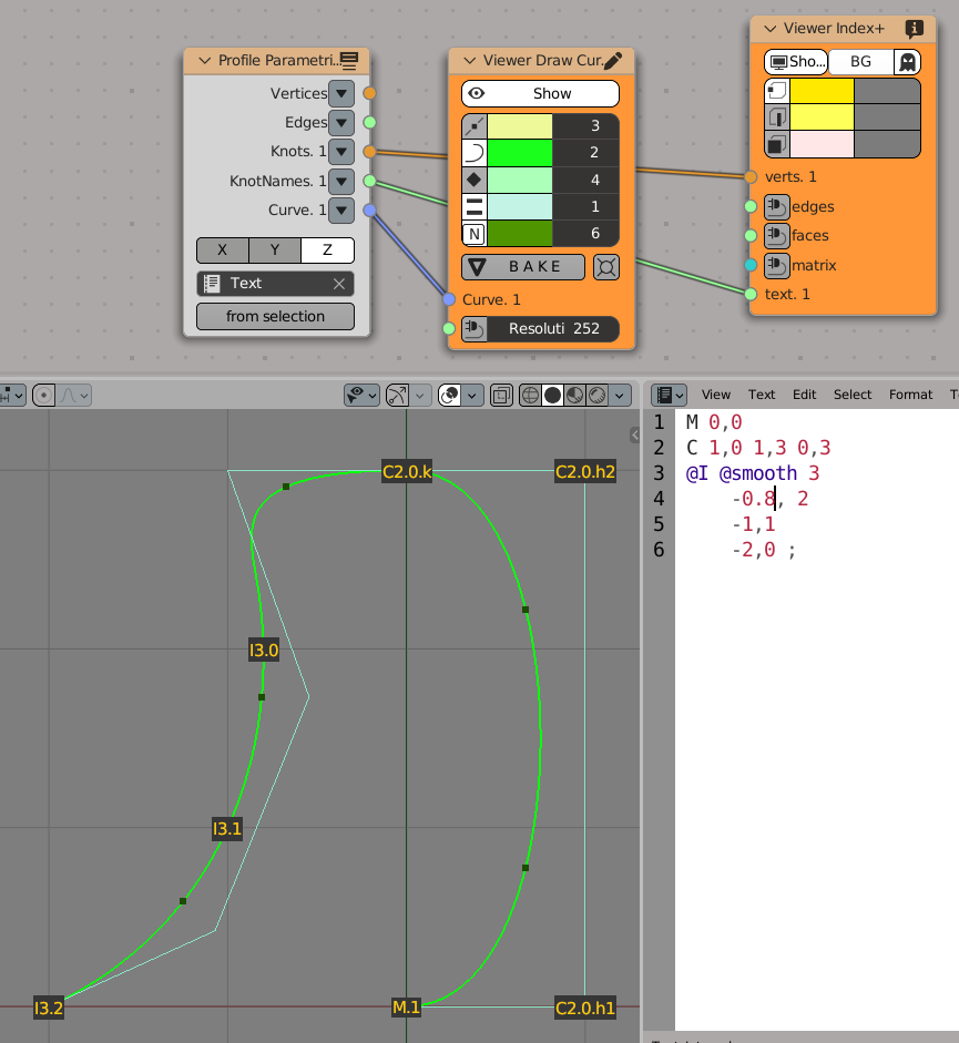
M 0,0
C 1,0 1,3 0,3
@I @smooth 3
   -0.8, 2
   -1, 1
   -2, 0 ;

Gotchas¶

The update mechanism doesn’t process inputs or anything until the following conditions are satisfied:

All inputs have to be connected, except ones that have default values declared by “default” statements.
The file field on the Node points to an existing Text File.

Keyboard Shortcut to refresh Profile Node¶

Updates made to the profile path text file are not propagated automatically to any nodes that might be reading that file. To refresh a Profile Node simply hit Ctrl+Enter In TextEditor while you are editing the file, or click one of the inputs or output sockets of Profile Node. There are other ways to refresh (change a value on one of the incoming nodes, or clicking the sockets of the incoming nodes)